This article comes with a pbix file: DAX - From the Trenches.pbix

This article is inspired by one of the latest DAX challenges I faced. This article contains DAX at the end and describes how I got there. I follow this process when facing a DAX challenge I cannot solve within 60 minutes.

This process is simple:

1. Understand the challenge (the business requirement)
2. Understand the model (if there is one)
3. Visualize iteration depth and iteration width using the matrix visual
4. GO – safe the world

Since I started using DAX to create measures, I learned that a solution evolves from passing two phases: problem understanding and problem solving. When looking back on all the DAX measures I created over the last years, it becomes evident that the most difficult ones (difficult does not necessarily mean complex) have been the ones where

I did

• not fully understand the problem, meaning the business requirement or
• not pay (enough) attention to detail or
• not know (enough) about the mechanics of DAX

Over time, some things have changed, I have become older and learned some mechanics. Unfortunately, there are still difficult DAX measures. In this article, I’m not focusing on DAX mechanics. Here, I’m focusing on the first two aspects: understanding the requirement and paying attention to detail.

The next sections of this article describe the process I’m following in more detail. To me, it’s very important to understand the requirements. Often, there are nuances in the phrasing that can have a great impact on the DAX.

But before I delve into the process, I think it’s necessary to provide an introduction to the professional setting where I conjure DAX magic. The Power BI landscape of our organization comprises many thousands of Power BI datasets. My colleagues and I have only seen a fraction of these datasets and know fewer by name. Some datasets are huge, some are small, some have a complex data model some don’t. Most of the datasets are behaving well. The point is that I do not know every dataset from the inside out. Keep this in mind when I introduce you to the analytical outline.

But now to the process.

After 60 minutes without creating a solution, I ask my colleagues for an analytical outline. Creating the outline may seem overhead, but it helps to focus on the solution and to avoid misunderstandings. This outline comprises:

1. Overall analytical target

   A short description of the analytical goal. Sometimes, this goal is a scalar value; sometimes, it’s about reducing the rows showing up in a visual; sometimes, it combines filtering and creating a scalar value.

2. Data interaction

   Basically, this is about slicers (or filters), as slicers are the most obvious way a user interacts with data. When writing DAX statements, I always imagine slicers as a means to filter the number of rows passed to the numeric expression, the formula that calculates the value.

   My imagination sometimes opposes the user's expectations because the existing report design does not match DAX reality.

   When discussing data interaction and the effect on the DAX statement to have a clear understanding of the following

   • What happens if more than one value is selected?
   • What happens if no value is selected (no slicer selection means all values are selected)?
   • Are the values inside a slicer representing all possible values, or are the visible values affected by measures or filters?
   • When “removing” an existing filter using a filter modifying function like ALL inside a CALCULATE, do I have to consider filters or measures that reduce the visible items inside a slicer?

   I notice that data interaction is often neglected when a requirement is formulated. This happens because we tend to focus on the most obvious. Often, we present a subset of data using a matrix or table visual, and based on the data, we ask for a DAX statement to calculate a measure.

3. A visualization of the expected result or behavior

   From my experience, it’s not the numeric expression that is complex. Most of the time, passing the exact number of rows to the numeric expression adds a lot of complexity to measure creation. To understand this complexity, I use the Matrix visual. The Matrix visual allows me to arrange all the relevant actors (table columns and measures) to be considered in a single visual.

   Forcing my colleagues to visualize their challenge in the form of a matrix visual when they need a measure to be visualized as a bar chart can be challenging; believe me 😊 But from my experience, it’s worth going the extra mile that sometimes feels like a fight. Maybe I will explain the rectangular data shape that feeds each data visualization of Power BI in a future blog article.

   I add all columns to the rows bucket of the Matrix visual that defines the measure's granularity (iteration depth) and all the columns to the columns bucket that defines the iteration width.

This chapter contains the business requirements of the challenge I mentioned above. It’s refined and can be considered the starting point for creating the analytical outline.

Assumption: You are a Business Analyst working for a company where you analyze business objects called "Item."

The business objects reveal insights when you look at the object's development over time (yes, you are right - a simple line chart for data visualization can help), but please wait - there is more ... It requires more explanation to understand the DAX challenge(s) better.

The business application that stores the objects initially provides a feature that allows users to define a set of rules (SOR). One set of rules can then be applied to one or many instances of an item. Not only can one set of rules be applied to one or many instances of an item, different sets of rules can also be applied to a single instance of an item. Each application of a SOR creates a new timeline. To rephrase the above a little:

• One or many SORs can be applied to one instance of an item
• One SOR can be applied to different items

A set of rules not only groups rules but also represents learning. For this reason, comparing results through applying different SORs to an instance of an Item will reveal a threat or an opportunity. Because learning happens as time goes by (at least most of the time :-) ), SORs can be ordered - the higher the order number, the more learning.

To refine analysis or reduce the amount of data to only an interesting portion of data, a business analyst wants to apply the three rules (conditions) below:

• Rule 1: Keep rows when only one of the selected SORs is assigned to an item.

• Rule 2: Remove rows from a Matrix visual when the Lifetime-Value (LT-Value, LTV) is above an absolute threshold.

  This rule removes the entire timeline defined by the combination of an item and an individual SOR when the sum of measurements across the timeline is above a given threshold.

• Rule 3: Remove rows from the Matrix visual that are above a relative change. Apply this rule only when two SORs are assigned to an item.

  This rule removes the combination of an Item and all SORs when none of the changes between two SORs is above or equal to a given threshold. If a single change is above or equal to the given threshold across all the time units, both timelines (item1/sor1 and item1/sor2) are kept otherwise, both combinations (item1/sor1 and item1/sor2) are removed.

I learned this through all the years: I need an example.

The next sections show an analytical outline. On rare occasions, it might take us (my colleagues and I) longer to create this outline than creating the DAX, but still, I consider this invaluable. It helps to avoid misunderstandings and, of course, is an essential part of the documentation of the data model. Each of the following sections closes with a comment. This comment is not part of the outline. It just adds some thoughts from writing this article.

The analytical outline I present in the following sections is redacted but not shortened. Nevertheless, sometimes it is shorter, sometimes it’s much longer. Sometimes, the answer is not only a DAX statement. Instead, the answer comprises multiple DAX measures and data model changes.

Filter out all rows from a Matrix visual that do not meet the above-mentioned business rules.

Comment: This is good, as the Matrix visual is the analyst's data visualization type. Nevertheless, even if the user wants to use the measure in a different data visualization type, I use the Matrix visual to “understand” the DAX I have to write.

Active Slicers: slicers are used to

• Select one or two SORs

• slicers are used to filter down the items (attributes of an item), I omit this in the example as this does not affect the measure, only the number of rows (the items) that are visualized

• A slicer is used to narrow down or expand the range of the timeline

  Regardless of the selected timeline, the rule “Above an absolute threshold” has to consider the complete lifecycle of an item.

Report level, Page level, and visual level filters are not in place.

Comment: Because only if one or two SORs are selected reasonable content can populate the matrix there must be a check how many SORs are selected in the slicer.

This part of the process is the most important one because it directly relates to the DAX I write.

The next picture shows a Matrix visual without any rules applied – it’s the baseline. The content is simplified, in reality, there are more columns and much, much more rows.

From the above image, we can learn that an analyst decides to compare sor1 and sor3.

The next picture shows the rows that will be removed from the matrix visual based on the rule "Condition 2: Remove when LT-Value is above Absolute Threshold” with an absolute threshold of 15" the two lines of Item i2 will be removed:

The next picture shows the application of “Condition 3: Relative Change above threshold” to item 1. Rows that will be removed or kept from the matrix visual based on the 2nd rule "Relative Change Threshold above 30%.” I omitted two checks for Item i1 for better readability.

Comment: Creating the “visual” explanation can result from a workshop spanning multiple hours to multiple days. This depends on the complexity of the underlying data model.

Before I delve into some DAX I want to explain the environment where I write or optimize DAX and why I think there is a difference between writing/optimizing and designing DAX. The difference between writing and designing DAX:

• Writing DAX: Write the best DAX possible without changing the model on a given DAX engine.
• Designing DAX: Change everything, the model, the DAX engine, and write the best DAX possible. Changing the DAX engine can mean migrating from SQL Server Analysis Service 2016 to a Fabric 256 capacity.

Sometimes, writing DAX is impossible because the slow DAX is optimal for the given environment. But also, sometimes, designing DAX is not possible for many reasons. Destroy expectations as soon as possible because otherwise, there is no time for a plan B. Sometimes, I face restrictions that can not be changed, at least not immediately. It is necessary to adapt to these restrictions and communicate how they will affect a solution. Of course, depending on the importance of the challenge we have to tackle, it can be possible to have a side step and import 100s of millions of rows to a Power BI dataset only to showcase the effect of windowing functions on performance. If we operate on a tight budget and a short time frame, we can only do what must be done to survive the next release.

Most of the time, when I’m tasked with writing or optimizing a DAX statement, I did not create the underlying data model. Creating the optimal DAX statement requires (at least) some understanding of the data model. I do not need to understand each column and every table, but it’s essential to understand the meaning of the columns on the one-side of the relationship of the affected tables. It is crucial to understand how business analysts refer to these keys and how they are “called” from a business perspective. If you wonder if this can be a problem - yes it can. A data model is exposed to continuous change, adapts faster than the documentation, and an item is called an item even if the key no longer represents an item but instead a version of an item.

My advise, be careful with the keys, the columns of the one-side of a relationship.

The next picture shows the data model. It's nothing special:

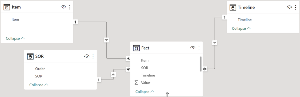
Some facts about the real dataset:

• The number of unique objects or items is ~1.5M (and growing). This makes it a larger dimension table; in reality, items bring a couple of attributes.
• There are ~100K SORs (and growing); a SOR has many attributes.
• Timeline "tracks" the development of items. Some items are old but still active. On average, 30 time units form the timeline per item.
• On average, an item has 20 SORs assigned.

The item's or SOR’s attributes are irrelevant to the challenge(s). The attributes, when selected, are used to reduce the items or the SORs. and for this reason, it's very simple: I purge them from the sample data :-)

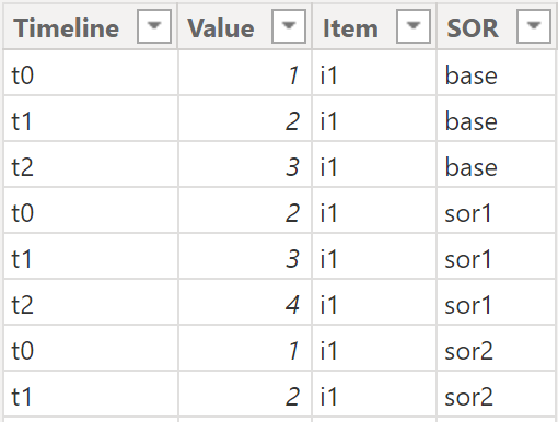
The following picture shows fact data. Please be aware that the fact table is not stored in a wide format. Of course, it's stored in long format. I only visualize the fact in the wide format for better readability:

The next picture offers a glimpse into the real world:

💡 From now on, whenever you see DAX it’s about calculating a measure. Everything you read in this article is about measures, when it’s about calculated columns I will explicitely mention calculated columns.

When I’m on my way to write a complex statement, I always start with a mock-up using pseudo code. This helps me to stay focused, I adapt this mock-up when I make progress or when I realize complexity is growing.

From my understanding of the requirement derived from the analytical outline and the discussion with the business analysts, DAX that performs the tricks below is required:

the Measure =
var noOfSOR = Check_Condition1_NoOfSelectedSORs
return
if noOfSOR <= 2
        , var Check_rule2_LTVisAboveAbsoluteThrehsold = IF(… , TRUE() , FALSE() )
        var Check_rule3_ChangeAboveRelativeThreshold = IF(… , TRUE() , FALSE() )
        return
        IF( Check_rule2_LTVisAboveAbsoluteThrehsold 
                        && Check_rule3_ChangeAboveRelativeThreshold
        ,       SUM( Fact[Value] ) -- the simple numeric expression
        , BLANK() -- removes unwanted rows
        )
        , "hint that only 1 or 2 SOR can be selected"
)

Even if it’s not obvious, the above measure contains, all three conditions:

1. Check_rule1_NoOfSelectedSORs a numeric value that allows to check if not more than 2 SORs are selected
2. Check_rule2_LTVisAboveAbsoluteThreshold a boolean value that checks the business rule “above an absolute threshold”
3. Check_rule3_ChangeAboveRelativeThreshold a boolean value that checks the business rule “above a change threshold”

The final measure is “the measure”, but before I explain the measure I talk about the components that make the measure a complexer measure.

Basically, the counting of selected values is simple, I assume we all use something that looks like the DAX below:

# of Selected SORs = 
COUNTROWS( VALUES( 'SOR'[SOR] ) )

When sor1 and sor3 are selected the measure above returns 2, simple like that. But there is more. If we are looking closely at the the requirements of condition 1 and 3 we have to count/determine the number of assigned SORs in the context of items.

The requirement “keep the row when only one of the selected SORs is assigned to an item” and “change above relative threshold” requires more than the count of the selected values from a slicer. Considering the measure execution for item i5 with only one SOR assigned a more subtle measure is required, one that returns 1. To determine the change between sor1 and sor3 it’s also necessary to respect the context of the item.

I often encounter challenges that require knowledge of a set of column values, here it’s the set of SORs in the context of a second column, here it’s the item colum, but also in the context of the fact table. For this reason I call this column values a contextual set. In my mind, a contextual set defines a group of items from a given table/column within a (partial) filter context, this partial filter context is defined by the column item. I need names for a problem, because otherwise I tend to loose focus. If you want a more fancy explanation, go to Quora and look for “Why do demons keep their real names a secret?”

The following DAX statement returns the contextual set of SORs for an item. This DAX code is used in various measures of course without the TOJSON wrapper:

helper ContextualSet = 
TOJSON(
    //the contextual set: the set of SORs in the context of an item
    WINDOW(
        -1 ,REL , 1 , REL
        , SUMMARIZE(
            ALLSELECTED( 'Fact' )
            , 'Item'[Item]
            , 'SOR'[SOR]
            , 'SOR'[Order]
        )
        , ORDERBY( 'SOR'[Order], ASC )
        , DEFAULT
        , PARTITIONBY( 'Item'[Item] )
    )
)

I assume you are familiar with the terms Evaluation Context and Filter Context. I think of these terms as concepts that are applied when a measure is evaluated. We are used to modify the filter context by using DAX functions like ALL and REMOVEFILTERS. Because a measure returns a scalar value, I also imagine that the two concepts are affecting a cell. I admit that it can be challenging to spot the cell, especially when looking at data visualizations like a bar chart or the card visual. Trust me - the cell is there!

Rule 2 - LT-Value is Above Absolute Threshold

But then there are requirements where we do not need to modify the filter context to calculate a value like a Year-to-date value or a ratio. Instead, it becomes necessary to prevent the calculation of a numeric expression either for a single cell or as in this DAX challenge for a combination of column values across a fact table: item and SOR.

The following images shows the fact table with highlighted rows:

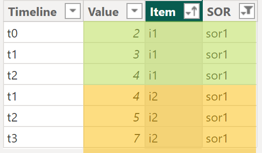
Based on rule 2 “Remove row when LT-Value is Above absolute threshold” the rows of item:i2 | SOR:sor1 (highlighted orange) must not appear in the Matrix visual when the absolute threshold is 15 or below because the LT-Value of i2|sor1 equals 16.

The next image shows all data with no rule applied visualized using the Matrix visual:

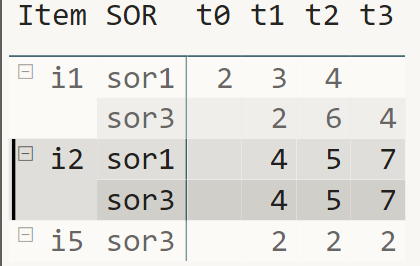
Because the LT-Value of i2 | sor1 is 16 the row must not appear. Unfortunately there is no “hide-row-if” option for the matrix or table visual. But we know that a row is automatically hidden when all the values of that row are blank. We have to make sure that for all of the three values the measure must return BLANK and Power BI takes care of hiding the row.

Even if the check can be easily computed by removing the timeline table from the filter context I think of this kind of iteration

IterateAcross_AllAvailable_SumOf

To perform the check theoretically it’s necessary to iterate across all available timeline items and sum the values. I call the number of iterations that must be performed to execute the check: iteration width. Of course, this type of iteration can be replaced by removing any filter of the timeline table that contributes to the filter context.

The DAX implementation becomes simple, see the DAX statement below:

Check_rule2_LTVisAboveAbsoluteThrehsold = 
//the absolute threshold
var absoluteThreshold = [Absolute Threshold Value]
return

//check if the value across the complete timeline is below the absolute 
//threshold. 
//a consideration might be to bring this "lifetime" value 
//to the item table, this might affect the granularity of the item table 
//if this value is implicitly affected by the SOR applied. 
//considerations like this might have a great impact on the 
//data processing and data loading happening further upstream
IF(
    CALCULATE(
        SUM( 'Fact'[Value] )
        , ALL( 'Timeline' )
    ) <= absoluteThreshold
    , 1 //below absolute threshold
    , BLANK() //above absolute threshold
)

Rule 3 - Change Above Relative Threshold

The application of this rule is more complex than the application of rule 2. This is because of the fact that this type of “rule” needs to combine the “contextual set” of SORs with the iteration across all the selected timeline items to calculate the change between the later SOR with the previous SOR. The following images highlights item i1 and both selected SORs:

Remember Rule 3: Hide i1 | sor1 and i1 | sor3 when there is no change that is above a change threshold, or less technically, hide two rows. We already know that this can only be achieved when each “cell” is blank. Because both “rows” must be hidden a measure must be evaluated 4 times per row or 8 times in total, unfortunately DAX does not provide an “exit” from an iteration when a given condition is met, this means the check must be performed as fast as possible.

The next image is visualizing the eight evaluations to perform the check:

The evaluation of measure is cell-based and is performed independent from an adjacent cell. Basically, this is good, but sometimes there are requirements that demand some creativity. The next image shows the important part of the measure “Check_rule3_ChangeAboveRelativeThreshold”, here the measure “helper ChangeAboveRelativeThreshold” is visualizing the calculations but only for the timeline item t0:

I think of this type of iteration as

IterateAcross_AnyOfDataDriven_Expression

All measure executions need to “know” if any of the expression evaluations (comparison of the two SORs per item/timeline) meets the condition. I’m pretty sure that there are many approaches how this check can be performed. I learned that unpivoting the SORs performs very well. What I mean by unpivoting is explained by the next to images, the first image shows data from the fact table:

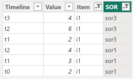
Within the measure “Check_rule3_ChangeAboveRelativeThreshold” this is happening:

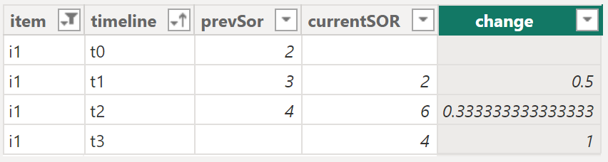
I realized that unpivoting the SORs and calculating the change as virtual column performs very fast. The DAX needs a FILTER on the change column comparing the change with the “Change Threshold.” All this is wrapped into COUNTROWS to determine if there is any change above the “Change threshold.”

There is a table “helper the unpivoted table” that creates an unpivoted table. I often start with creating a virtual table to get an idea what I have to do before I put the DAX into the measure. For this reason be aware that the DAX of the table and the measure are different.

One universal truth about DAX is the lazy evaluation of variables and the lazy evaluation of conditions inside the IF statement. Lazy evaluation means that the expression will only be evaluated if required.

The DAX snippet below is the final measure “the measure.”

the measure = 
-- sanity check
var numberOFSORsSelected = COUNTROWS( ALLSELECTED( 'SOR'[SOR] ) )
return

IF( numberOFSORsSelected <= 2
    -- this determines all the SORs of an item in the given context and count the rows.
    -- this is required to keep the row of item i5 and SOR s0r3
    , var numberOfSORsApplied = 
        countrows(
            window(
                -1 ,REL , 1 , REL
                    , SUMMARIZE(
                        ALLSELECTED( 'Fact' )
                        , 'Item'[Item]
                        , 'SOR'[SOR]
                        , 'SOR'[Order]
                    )
                , ORDERBY( 'SOR'[Order], ASC )
                , DEFAULT
                , PARTITIONBY( 'Item'[Item] )
            )
        )
    return
    IF( numberOfSORsApplied = 1 || ( [Check_rule2_LTVisAboveAbsoluteThrehsold] >= 1 
&& [Check_rule3_ChangeAboveRelativeThreshold] >= 1 )
        , SUM( 'Fact'[Value] )
        , BLANK() -- removes the row from the matrix, because null rows are "hidden" by default
    )
    , "Select only one or two SORs"
)

For the above lazy evaluation means that

• Check_rule2… will only be evaluated if there are 2 SORs applied to one item. When conditions are combined using the logical OR operator ( || ) the second condition will only be evaluated if the first condition is FALSE. The evaluation of the second condition only starts when first condition is FALSE, when more than 1 SORs are applied to an item.
• Check_rule2… and Check_rule3 are combined by the logical AND operator (&&). If conditions are combined by AND make sure that the easy condition is the first condition to be checked. Easy means, fast.

Hopefully, you enjoyed reading this article, even if it was a little lenghty.